Employing phase metrics and spectral power to understand ocean wave direction, speed and strength from accelerometer based sea-level data from oceanic buoys

Introduction

• Oceanic Buoys and accelerometer data
• Spectral decomposition
• Identification of coherence

Buoy accelerometer data

If you haven’t yet seen a random floating bulb in the middle of the ocean, that bobs up and down blinking ever so silently in the vastness, you’re in luck! While there are many types of buoys, we would be considering the data generated from a specific one of these, the Oceanographic Buoy!

Oceanic buoys equipped with accelerometers provide valuable data for studying wave dynamics, including their movement speed, direction, and intensity. This article will explain the basics of the theories involved and the process to achieve this understanding. In this article, we will discuss how to derive spectral decomposition from a given time-series, such as an Oceanic Buoy’s accelerometer data, to ascertain metrics associated with the cyclic events that may be present within the respective series.

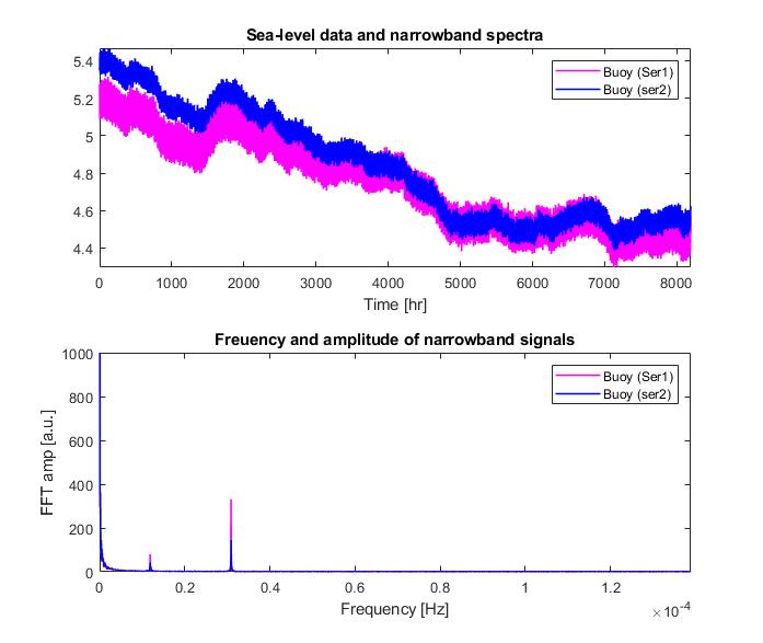
Accelerometers measure acceleration, which is the rate of change of velocity of an object. In the context of oceanic buoys, accelerometers record the buoy’s acceleration due to wave motion. This data is fundamental for understanding wave characteristics. In the given example, we have a record of buoy data over 8000 hours, which tabulates the sea level detected from the accelerometer movement, which can then be used to quantify wave fluctations, duration and intensity over time upon considering frequency, amplitude, and wavelength of the generated time-series. We can employ Signal processing techniques such as Fourier transforms and wavelet analysis to convert raw data into frequency-domain representations crucial for extracting meaningful information from accelerometer data.

Using fourier transform to extract useful data

Joseph Fourier, a french mathematician came up with the idea to decompose any given time-series as a function of infinite series sum of sines and cosines, which led to the development of the Fourier Transform. This transform can be computed on discrete or continuous time-series which could be ADC captured signals or real world signals respectively. Fourier transform represented as follows:

which can be computed digitally using the butterfly technique called the Fast Fourier Transform (FFT) algorithm, there’s a good reference article explaining Cooley and Tukey’s work by the way of implementation in MATLAB and Python.

Metrics to extract

We can use both the raw signal amplitude data as well as the decomposed frequency domain data from the buoys to extract the following information:

• Time-domain signal data
  • Average sea-level
  • Sea-level deviation between buoys and general bobbing noise / standard noise floor
  • Phase delays/ lag between waves
  • Correlation between the signals from the buoys
  • DAS beamforming for calculating wave sources (with multiple buoys 2+)
    • +bonus: An application to detect tsunami or strong currents
• Frequency-domain signal data
  • Prominent wave frequencies and associated intensities
    • +bonus: An application to calculate power generation ability for offshore energy harvesting

Usually, an array of several buoys are deployed in a given region to monitor the above mentioned metrics and more from other sensors, for this article, we will only consider the data from 2 buoys placed at a distance to obtain the above mentioned metrics.

Methodology

We would be undertaking the following tasks to obtain the metrics and understanding mentioned above:

• Filtering: to detect and remove any noise
• Statistical analysis
• Correlation analysis
• Fourier decomposition
• Spectral power analysis

Analyses

Preprocessing

These buoys are equipped with accelerometers, GPS for location, and usually other sensors for environmental parameters, such as a pressure sensor on the ocean floor to track water cloumn load above (Ex. DART program). Raw accelerometer data is often noisy. Preprocessing includes filtering, calibration, and alignment to ensure accurate readings. Additionally, GPS data helps synchronize the data from different buoys. In our example, we have accelerometer data from 2 buoys which we will filter with a Low-Pass, FIR butterworth filter designed using the filter design tool designfilt.

The choice of filter and respective bandpass and bandstop frequencies are highly dependant on the application, upon doing an FFT decomposition before filtering can show how the noise is dispersed and the choice of paramters can henceforth be made. For this signal data, we will choose the mentioned passband and stopband frequencies. For more details on Filtering and a complete guide, you may find [my guide on Filters][10] informative towards designing your own filter based on desired information, speed, resonance and noise constraints.

Tip: If you don’t know the sampling frequency and if have an idea of the signal duration t and N total samples, you can utilize the simple equation to obtain the sampling frequency OR use (max(data)-min(data))/(samples-1)

Tip: You can also use the GUI based filterdesigner tool to design the filter based upon your choice of parameters.

Tip: You can also utilize fvtool to visualize the frequency response of your filter.

% Sampling frequency [Hz]
fs = 1/(60*60); % since data was recorded every hour 

% Before filtering, we should remove any linear trends that are a part of this data, using a linear fit:
dtSig1 = detrend(buoy1);
dtSig2 = detrend(buoy2);

% Change in the trend of the sea-floor 
tChange1 = buoy1 - dtSig1;
tChange2 = buoy2 - dtSig2;

% Filtering out the lowest frequency signals 
filterLP = designfilt('lowpassfir', 'FilterOrder', 30, 'PassbandFrequency', .000030, 'StopbandFrequency', .000035, 'SampleRate', 0.00027778);

% Apply the filter to both raw signals
filteredSig1 = filter(filterLP, dtSig1);
filteredSig2 = filter(filterLP, dtSig2);

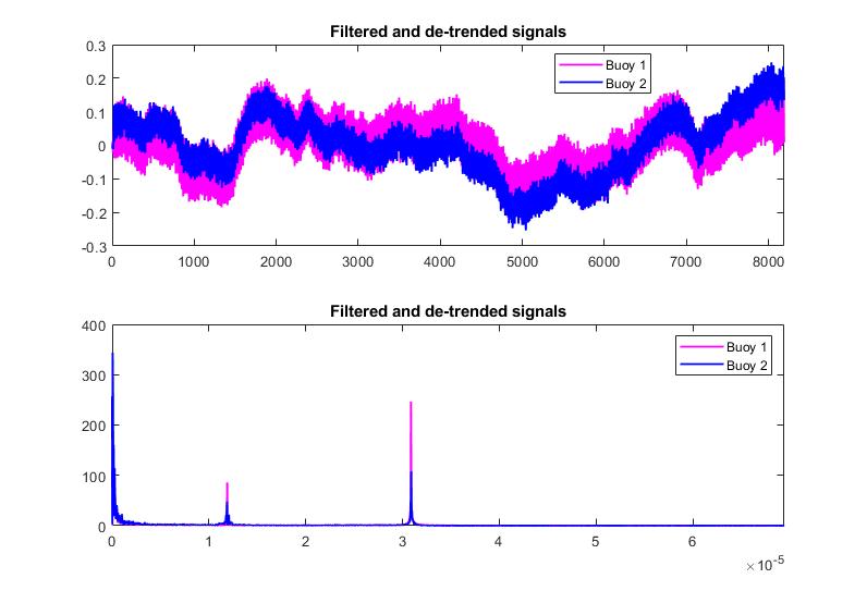
which gives us

Raw buoy signal data	De-trended and filtered data

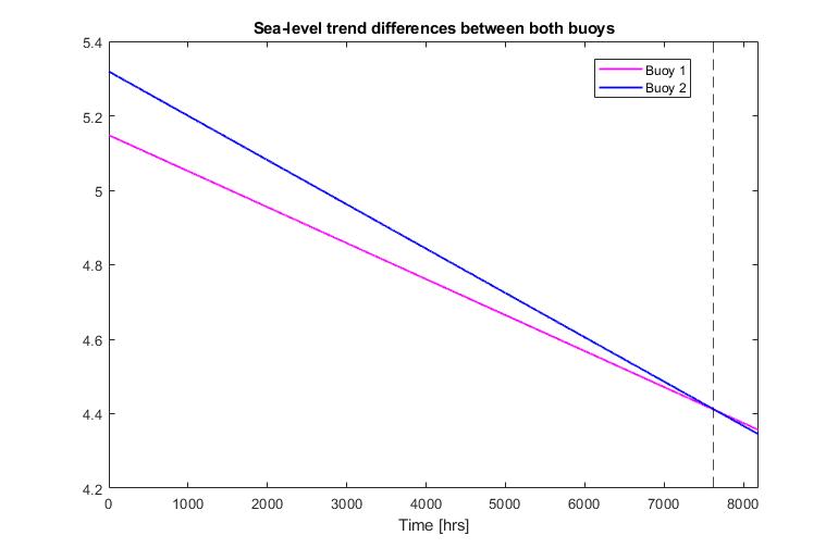
The linear fit for the identified trend was as follows, which can be obtained by simple DC subtraction from the signal. This data can be used to find out instances of time when multiple buoys (>2) are at roughly the same height and the sea-floor can be assumed flat, which can be utilized for 3 dimesional triangulation of other objects perceived via other sensors on all buoys. This has applications in position tracking via an array of buoys towards pressure, windspeed, object location estimation etc.

Statistical metrics

Now that our signal data has been rid of noise, let’s first determine the amount of signal power and quality, which can be ascertained using the Signal to Noise Ratio (SNR)

Tip: We can utilize the trapz function to obtain the total power in the signal along all frequency bins. It will be added twice (due the symmetrical output of fft, but that cancels out due to both numberator and denominator being scaled by 2). One can also use the more general pwelch method to

Now, let’s extract some simple metrics:

% Isolating the background noise data
noiseBuoy1 = dtSig1 - filteredSig1;
noiseBuoy2 = dtSig2 - filteredSig2;

% SNR
SNRbuoy1 = 10*log(trapz(abs(fft(filteredBuoy1,N)))/trapz(abs(fft(noiseBuoy1,N))));
SNRbuoy2 = 10*log(trapz(abs(fft(filteredBuoy2,N)))/trapz(abs(fft(noiseBuoy2,N))));

% Average wave-height
meanBuoy1 = mean(filteredSig1);
meanBuoy2 = mean(filteredSig2);

% We can check the background continuum sea-level buy subtraction and verify it using the mean difference,
sealLevelChange = dtSig1 - dtSig2;

% + Standard Sea-level flucations / Standard noise floor  
stFluctuations1 = 3*std(noiseBuoy1);
stFluctuations2 = 3*std(noiseBuoy2);

% Phase delays 
y1 = fftshift(fft(buoy1,N)); y2 = fftshift(fft(buoy2));
pad = 100; % To avoid frequency bins nears the end

[~,binIndex] = max(fftFiltSig1((N/2) + pad:end-pad)); % Padding 100 to remove noisey samples (plot this to see the samples considered for max)

phaseLag12 = angle(y1(binIndex+pad+(N/2))/y2(binIndex+pad+(N/2)));
phaseLagDegrees12 = (360*phaseLag)/pi; % Which gives => (lag in degrees/360)*(10hrs ~ approx. time taken to capture 1 cyle/ wavelength)

timeLaginHrs12 = (phaseLagDegrees/360)*(10); % time lag in hours of buoy 2 with respect to buoy 1 

% Correlation
coherenceBuoys = mscohere(dtSig1,dtSig2)
plot(wden(mscohere(dtSig1,dtSig2), 'modwtsqtwolog', 's','mln',3,'db4'))

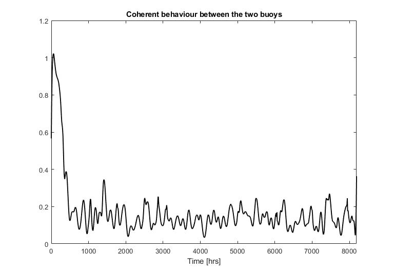
We can observe how the coehrence drops and is mostly low through the period that the buoys were tracked, showcasing that:

• wave activities for both buoys were independant of each other, hence
• both the buoys must be placed relatively far from each other to not record the same minor fluctuations

Application: DAS beamforming

[DAS][11] or Delay-And-Sum beamforming is a tehcnique used in medical technologies, conventionally, biomedical ultrasound, to [‘echo locate’] sources. This is done by using a phased-array of receivers, that add relevant delays to each transmitting source (for transmit beamforming) OR add relevant delays to each receiver depending on a ‘known location’ (receive beamforming) to transmit energy/ signals OR determine what’s happening at the ‘known location’, respectively. There’s a great article discussing the [developmental history of such algorithms][12]. Multiple sources can be echo-located if their signature frequencies are different.

Pertaining to Oceanic-buoys, if the location of the buoys is known (since they are actively deployed and maintained) and if we are able to have a good estimate of sea-levels from such buoys: receiving a large change (rise/ dip) in the ocean level on multiple buoys, can be utilized to receive DAS beamform the source of large rises/dips and predict the travelling direction of tsunami’s, which can be very helpful for disaster management in tsunami prone regions! Extant tsunami control programs, such as the DART program mentioned earlier, utilize ocean floor volumetric pressure as an estimate for tsunami’s, DAS has not been utilized for the same and a feasibility study is pending. (Perhaps I’ll do an analyses over publicly available datasets sometime…)

Frequency domain data

To understand ocean wave properties, accelerometer data is transformed into the time-frequency domain using techniques such as FFT as mentioned above. These methods reveal the most prominent frequency and intensity of waves over the whole period of data acquisition. Another method such as the STFT (Short Time Fourier Transform) can be utilized towards identifying the how the frequency or the intensity of waves changed over-time, hence additional time resolution can be achieved. My matlab code for STFT can be found [here][13]. You may also find this python method much easier and direct:

# Function for Short-Time Fourier Transform (STFT) in Python
import numpy as np
from scipy.signal import stft
import matplotlib.pyplot as plt

# Assuming the signal is a 1D vector
def stftSignal(np.array(signal), t, fs):
    f, t, Zxx = stft(signal, fs, nperseg=200, noverlap=100)
    plt.pcolormesh(t, f, 20 * np.log10(np.abs(Zxx)))
    plt.title('STFT of buoy')
    plt.ylabel('Frequency [Hz]')
    plt.xlabel('Time [s]')
    plt.show()

Looking at the FFT data produced, we are able to identify some primary features:

• The most prominent cyclical behaviour is at 30.8e-6 Hz, which is roughly once every 8.9 hrs, the second peak is at 23.5 hrs
• These signify two VERY clear periodic events: one that happens every day, the other twice a day
• Buoy 1 has a better accelrometer sensitivity (higher values for similar FFT bins)
• Sea-level change also prominently showcases

Conclusion

Understanding accelerometer data from multiple oceanic buoys and identifying coherence between waves and wave movement speed, direction, and intensity involves a combination of accelerometer theory, wave theory, and signal processing techniques. The process of data collection, preprocessing, time-frequency analysis, and coherence analysis allows us to extract meaningful information from the data, aiding in the understanding of ocean wave behavior.

Other matlab or Python code relevant to this project can be found in [my git repos][14] for computing the f

• Filtering
• Fourier transforming
• SNR calculations
• Coherence
• Visualizations

Takeaways

• Filtering and extraction phase and speectral information from a time-series data in Python.
• An application of Oceanic Buoy data towards identifying and analyzing Oceanographic metrics.

[10]: [11]: http://www.labbookpages.co.uk/audio/beamforming/delaySum.html [12]: https://signalprocessingsociety.org/publications-resources/blog/echo-time-tracing-evolution-beamforming-algorithms [13]: [14]: https://github.com/0-Kaustubh-0