Using wavelet cross-coherence on fNIRS data to investigate Inter-Neuronal-Syncing between Musician and Listener combinations
In this article we will explore
- What are Wavelet Transforms?
- What is a Cross - Wavelet Transform?
- What is fNIRS?
- What is Inter-Neuronal Synchronization
- Application of Cross-Wavelet Tranform to fNIRS data to obtain INS scores
- Relevant metrics from Musicians and Listeners
- INS t-maps
- Granger-Causality tests
- Regression ROC curves
- Statistical metrics & Visualization
What are Wavelet Transforms?
If you are here you probably understand how any time-series is made up of several superimposing frequency components. Joseph Fourier brilliantly posited in the 18th century that all time series or functions could be decomposed into a series sum of sines and cosines, a breakthrough which (with some additional rules applied) led to the developement of the Fourier Transform! This tool can be used to decompose any continuous signal that we record, into it’s consittuent frequency components (sum of Sines and Cosines with associated ‘weights’/ ‘coefficients’) over the whole signal (we’ll come back to this…).
Wavelet Transform is a technique developed by Ingrid Daubchies which does the same thing but with an additional, most useful functionality: it is able to decompose the signal into it’s constituent frequency components with time-resolution! i.e. not only can you tell which frequency components arose in the signal, you can tell when they arose. This is highly useful in determining spectral events as a function of time, in the field of Biomedical Signalling, Geology, Astronomy etc.
For example, if there is a time-series, x, its continuous-wavelet-transform (CWT) is given by:
This computation can be acieved within MATLAB, using a one-line function in the Wavelet toolbox, by additionally specifying the sampling frequency fs for x:
1
[cwt_X, fVec] = cwt(x, fs);
which provides wavelet coefficients cwtX and the associated frequency vector fVec as the output. We should keep in mind that cwtX is real-valued and hence contains vital phase information as well. The phase information can be utilized in fields such as geology to contour bandwidths with common pahse and identify delays between different cyclical frequency components.
Introduction to Cross Wavelet Analysis
Cross wavelet analysis is an extension of the wavelet transform that allows us to compare and analyze the relationships between two time-series signals in the time-frequency domain. It helps us identify common patterns and interactions between two signals. The cross-wavelet is computed by multiplying the wavelet coefficients obtained from the Continuous Wavelet Transform from time-series x1 with the conjugate wavelet coefficients of x2 as shown below:
which can be computed in MATLAB using:
1
2
3
4
5
% Method 1: Using the conjugate method
XCorr = cwt_X1*conj(cwt_X2);

% Method 2: Using the in-built function
XCorr = wcoherence(x1,x2);
where XCorr posses the cross-correlation values. I personally prefer the 1st method as the it allows us the opportunity to:
- Inspect the indivdual spectral decompositions
cwt_X1, cwt_X2and - Do a inverse cross-wavelet analysis, such as
XCorr_inverse = (cwt_X2)*conj(cwt_X1);which allows us to further inspect which signal may have influenced the other, by employing the Granger-Causality test.
Tip: Plotting (XCorr, fVec) may be an issue with plot(), you may want to use imagesc() instead.
What is fNIRS?
fNIRS or functional Near-InfraRed Spectroscopy, is a non-invasive optical imaging technique using absorption spectra in the range of 700 nm- 1 µm to determine bloox oxygenation differences. Changing heamoglobin concentrations correlate with brain activity and can be used to monitor the same in the brain regions under the sensor closest to the skull.
How do we infer Inter-Neuronal-Synchronization(INS) from Cross-Wavelet Tansform
INS is a value that determines the correlation of the brain activity among two participants, it is calculated using cross-correlation between the brain signal data otained from each participant. This correlation can be caluclated using you guessed it, cross-wavelet-correlation. The data obtained from cross-correlation is averaged between a given bandwidth of interest, which usually coincides with the highest power spectral density that is common to both spectral decompositions. The data averaged within this bandwidth, is the INS score, which is able to identify brain activity correlation with time resolution, hence giving us the ability to map neural responses between two patients over time.
Let’s say we have a fNIRS time-series data captured from a single sensor on person A’s scalp, and another set from another sensor on person B’s scalp, named x1 and x2 respectively. Then the INS score couold be given by:
1
2
3
4
5
6
7
8
9
10
11
% Identify the bandwidth of interest (BOI):
% - literature
% - observation
BOI = [bwLow bwHigh];

% Find where the BOI is present within fVec
[~, bwLowIdx] = min(abs(fVec - BOI(1)));
[~, bwHighIdx] = min(abs(fVec - BOI(2)));

% Calculate INS between bandwidth of interest
INSscore = mean(XCorr(:,bwLowIdx: bwHighIdx), 2);
Applying cross-wavelet to extract INS coherence data between Musicians and Listeners
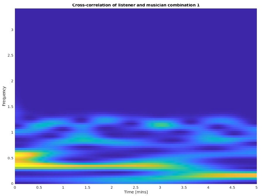
From a sample fNIRS dataset of 3 Musicians(Mn) and 3 Listeners(Ln), we are able to investigate the INS between the Musician-Listner combinations as well as Listener-Listener combinations (If we choose to compute auto-correlation and inverse correlation, we get 6*6 = 36 combinations). Observe the cross-wavelet coherence plot I created below ustilizng imagesc (why not plot? : due to very high sample density) and pcolor. This creates a heatmap with
- Time on the x-axis
- Frequency on the y-axis
showcasing how high OR low the correlation between the signals can be overtime and over diferent bandwidths.
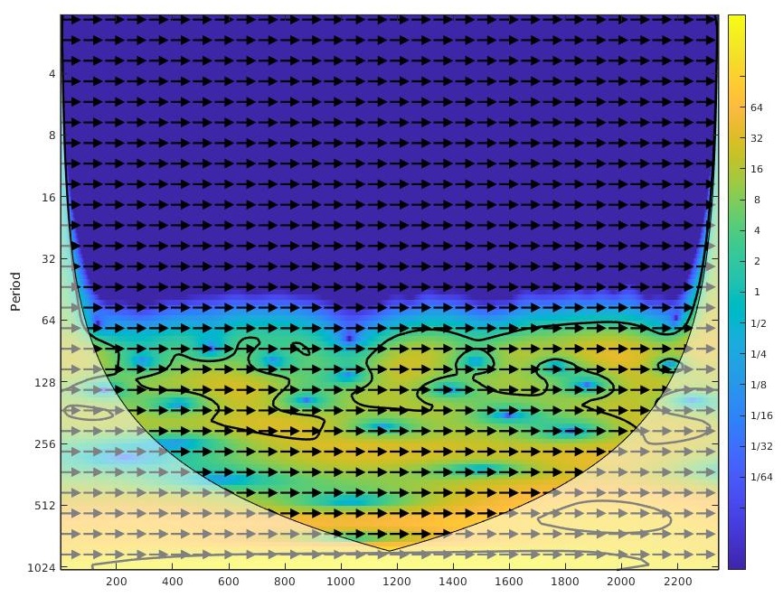
or as below if you utilize the direct XWT function from the MATLAB library created by Grinstead A. et al,
NOTE: This funciton incorporates a feature to generate contours around regions with high cross-correlation which maybe helpful in identifying trends within a given bandwidth or across bandwidths.
Extracting the metrics
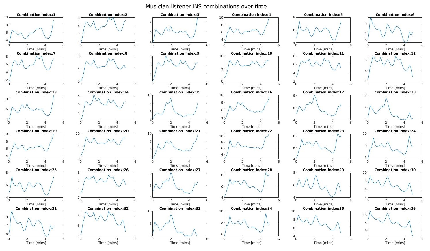
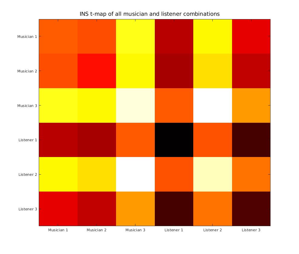
I identified the bandwidth of interest for investigating INS between the Muscian and Listeners to fall between 0.1 - 0.7 Hz. Now computing the average over XCorr values across all frequencies in this bandwidth, we can to derive the INSscore for a set of cross-correlation combinations. We can aso create a heatmap for the several combinations by calculating the max() over all correlation values over time for each combination.
We observe:
- There is a high coherence between some ML combinations and LL combinations
- There is a low coherence observed for MM combinations (as they were separate instances of fNIRS recordings)
- The INS is not stable and may fluctuate either way over-time (which may depend on the type of music, listener’s attention and receptivity or environmental acoustics)
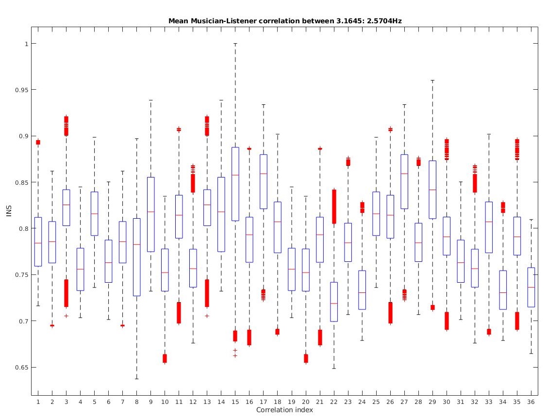
Looking at the data, one may find it to be skewed (since the bandwidth of interest selectively filters out frequencies that exhibit low cross-correlation, it also cannot filter out low correlation within the bandwith of interest at random time intervals), hence to remove skewnessm, we can Log transform the mean data.
This transformation reduces the skewness on the INS values and we can now derive mean INS and its variance overtime within this set bandwidth for the several unique combinations of Musicians and Listeners. More such plots could be generated for other bandwidths to identify which bandwidths have consistently low INS scores, and the mean within those bandwidths can be used to Normalize this data, for relative comparison between different combinations to be more precise.
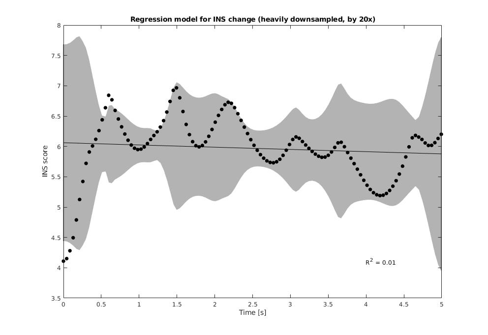
To understand whether this relationship between INS among two participants is related to/ dependant on / can be predicted by time, we can run the INS through a Regeression Analysis and draw the CI (Confidence Interval) for the same, it took me some effort to get this function working the way it does, so enjoy!
From this, we can conclude:
- Inverse correlation between any two signals has a symmetric response, implying there is low-noise in this dataset.
- Even listeners listening to the same musician can have a higher INS than the INS with the respective musician they are both listening to.
- [Negative result] The INS values are completely independant of time: musical synchroinization may come and go (N limited due to datasset size).
Cross Wavelet data analysis on MATLAB
The following MATLAB code snippet, describes the complete process to obtain the metrics from the generated INS scores. All the functions can be found in my github repo XCorr/.
1
2
3
4
5
6
7
8
9
10
11
12
13
14
15
16
17
18
19
20
21
22
23
24
25
26
27
28
29
30
31
32
33
34
35
36
37
38
39
40
41
42
43
44
45
46
47
48
49
50
51
52
53
54
55
56
57
58
59
60
61
62
% Make sure you have the Signal Processing Toolbox and the Wavelet Toolbox  installed
% Addtional info can be found at: https://github.com/0-Kaustubh-0/XCorr#xcorr

%% Select the signals to send
function mainXCorr(sig1, sig2, fs)
    % Example function

    % Prepare the signals for X-correlation
    [sig1, sig2] = modifySignals(sig1, ...      % Raw signal data stack/ singular
                                 sig2, ...      % Raw signal data stack/ singular
                                 dsFactor,...   % (double) Downsampling factor
                                 trim);          % (double) Trimming length (signal should have same number of samples)
    % ***** NOTE : Signal stacks sig1, sig2 are returned as row vectors *****

    % Set Options
    createPlots = 1; % Create plots for CWT
    shouldNormalize = 1;% Normalize the data
    shouldLog = 1;% Log transform the data

    % Compute CWT with signal stacks: signal1, signal2
    [crossWT, crossWTReverse, fVec] =   computeCWT(signal1, ... % Signal stack 1 (nSignals, N)
                                        signal2, ...            % Signal stack 2 (nSignals, N)
                                        fs,...                  % (double) Sampling frequency
                                        createPlots);           % (string) Create XCorr | CWT | XWT plots

    % Run the analysis on the crossWT
    [meanNarrowbandCoherence, ...
        narrowbandCoherencePhase, meanNarrowBandCoherenceBlocks] =  meanCoherence(crossWT, ...  % Cross-wavelet data for all many-many:: sig1-sig2 combinations
                                                                    crossWTReverse, ...         % Reverse cross-wavelet data for all many-many:: sig2-sig1 combinations *** (In order with sig1-sig2) ***
                                                                    fVec, ...                   % Frequency vector
                                                                    t, ...                      % Time vector
                                                                    BandwidthOfInterest,...     % Bandwidth of interest for finding correlation ** Important to observe with
                                                                    shouldNormalize, ...        % Choose to normalize: Normalize the mean coherence to the maximum correlation value
                                                                    shouldLog, ...              % Log transform the data if skewed
                                                                    NWindows);                  % Number of windows

    % Plot selected graphs, options:
    %   - Boxplot
    %   - Line plot for each correlation
    %   - t-maps/ heatmaps
    %   - regression analysis (R-Squared with ROC plots)
    plotThis(option, ...                % Option to select the plot to create:
             sig1, ...                  % signal stack 1
             sig2, ...                  % signal stack 2
             meanNarrowbandCoherence);  % mean coherence values over specified bandwidth

    % Plots for windowed data depend on user need: plot for coherence between sig1 and sig 2 stacks by:
    % - signal window
    % - correlation between windows
    % -

end

% Auto-regression model
% varm fucntion
% for j = 1:9
%     ARm(j,:) = varm(meanNarrowbandCoherence(j,:));
% end

% Run Granger analysis
% function gctest
% h = gctest(meanNarrowbandCoherence(1,:), meanNarrowbandCoherenceReverse(1,:));
Takeaways
- What is cross-wavelet correlation
- How to apply it using MATLAB and infer correlation results
- An application of fNIRS data to study Inter-Neuronal-Synchronization
